← Back to the Front Page

Dynamic Mode Decomposition: Learning Linear Dynamics from Blinking Blobs

Dynamic Mode Decomposition (DMD) is a powerful technique for extracting coherent structures and temporal patterns from high-dimensional, time-dependent data. Originally developed in fluid mechanics, it has since found applications in fields ranging from neuroscience to video processing.

Unlike traditional dimensionality reduction, DMD approximates the full system dynamics using a linear operator. This makes it ideal for modeling, forecasting, and separating physical processes — even when the underlying system is nonlinear.

A Visual Example: Two Blinking Gaussian Blobs

To build intuition, we generate synthetic data from two Gaussian blobs located at different positions on a 2D grid. Each blob "blinks" (oscillates in amplitude) at a distinct frequency, creating a spatially structured, temporally evolving dataset.

Mathematically, the data forms a time series of 2D frames \( X(t) \in \mathbb{R}^{n_x \times n_y} \), reshaped into a matrix \( X \in \mathbb{R}^{n \times T} \), where each column is a flattened frame at time \( t \).


  def generate_blinking_blobs(T=100, nx=50, ny=50):
      x = np.linspace(0, 10, nx)
      y = np.linspace(0, 10, ny)
      X, Y = np.meshgrid(x, y)

      center1 = (3, 3)
      center2 = (7, 7)

      freq1 = 0.1  # slower oscillation
      freq2 = 0.25  # faster oscillation

      data = []
      for t in range(T):
          amp1 = 0.5 * (1 + np.sin(2 * np.pi * freq1 * t))
          amp2 = 0.5 * (1 + np.sin(2 * np.pi * freq2 * t))
          blob1 = amp1 * np.exp(-((X - center1[0])**2 + (Y - center1[1])**2))
          blob2 = amp2 * np.exp(-((X - center2[0])**2 + (Y - center2[1])**2))
          frame = blob1 + blob2
          data.append(frame)
      return np.array(data)  # shape: (T, ny, nx)

Once the data is generated, we reshape it into a matrix where each column is a time snapshot, and apply the DMD algorithm step by step.

The DMD Algorithm: Step by Step

Given a sequence of states over time, the core assumption of DMD is that there exists a (possibly low-rank) linear operator \( A \) such that: \[ X' \approx A X \] where \( X \) and \( X' \) are two sequentially shifted data matrices.

To compute \( A \), we perform the following:

Split the data: \( X = [x_0, \dots, x_{T-2}], \quad X' = [x_1, \dots, x_{T-1}] \)
Compute SVD: \( X = U \Sigma V^* \)
Truncate to rank \( r \): keep only the top \( r \) modes
Form the reduced operator: \( \tilde{A} = U_r^T X' V_r \Sigma_r^{-1} \)
Compute eigenpairs: \( \tilde{A} W = W \Lambda \)
Lift eigenvectors: \( \Phi = X' V_r \Sigma_r^{-1} W \)

The modes \( \Phi \) describe spatial structures. Their time evolution is governed by the eigenvalues \( \lambda \), where \( \omega = \log(\lambda) \) gives continuous-time dynamics.


  X = data_reshaped[:, :-1]
  X_prime = data_reshaped[:, 1:]

  U, S, Vh = svd(X, full_matrices=False)
  r = 10
  U_r = U[:, :r]
  S_r = np.diag(S[:r])
  V_r = Vh.conj().T[:, :r]

  A_tilde = U_r.T @ X_prime @ V_r @ pinv(S_r)
  eigenvalues, W = eig(A_tilde)
  Phi = X_prime @ V_r @ pinv(S_r) @ W

  # Filter out small eigenvalues
  valid = np.abs(eigenvalues) > 1e-10
  eigenvalues = eigenvalues[valid]
  W = W[:, valid]
  Phi = Phi[:, valid]

  omega = np.log(eigenvalues)
  b = pinv(Phi) @ X[:, 0]
  time_dynamics = np.array([b * np.exp(omega * t) for t in range(T-1)]).T
  X_dmd = Phi @ time_dynamics

Results and Visualizations

The outputs of the DMD process reveal both the spatial modes and how they evolve in time:

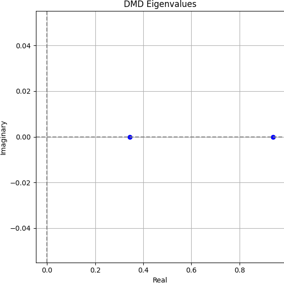
DMD Eigenvalues: Their location in the complex plane determines oscillatory vs. decaying modes.
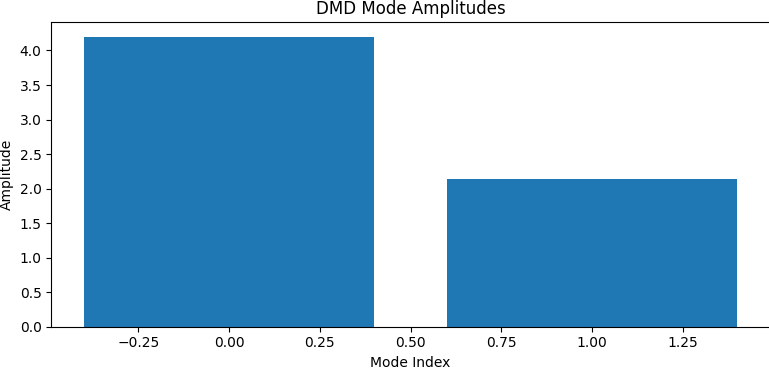
Mode Amplitudes: Initial energy in each mode (coefficients \( b_i \)).
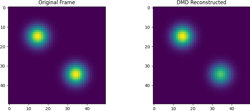
Reconstruction: Comparing the original data to the DMD model reveals fidelity.
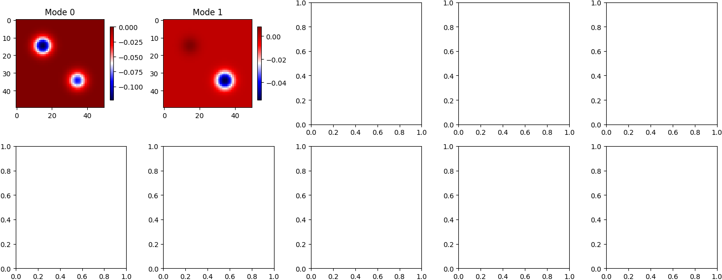
Modes: Show spatial patterns that persist across time.
Temporal Dynamics: Show how each mode oscillates or decays over time.

DMD Eigenvalues — **Figure:** DMD eigenvalues plotted in the complex plane.

DMD Mode Amplitudes — **Figure:** Initial amplitudes of the dominant modes.

Original vs DMD Reconstructed Frame — **Figure:** Comparison of true vs. reconstructed data.

DMD Modes — **Figure:** Spatial patterns of the top DMD modes.

Temporal Evolution of DMD Modes — **Figure:** Time dynamics of the five most active modes.

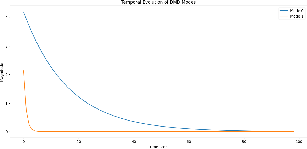
DMD successfully decomposes the blinking blob data into meaningful spatial modes and clean temporal dynamics. This simple experiment illustrates the method's ability to find structure in time-dependent data, even when no underlying equations are known. The linear nature of DMD allows for fast simulation, prediction, and interpretation — making it a versatile tool for modern data-driven science.

Analyzing Fluorescence Dynamics in a Simulated Cell Using DMD

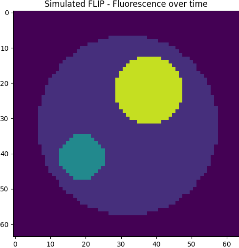
To demonstrate how DMD can uncover biological structure in image sequences, we simulate a simplified FLIP (Fluorescence Loss In Photobleaching) experiment on a model cell. This artificial cell consists of three compartments:

Cytoplasm: the main area of the cell, where photobleaching occurs gradually.
Nucleus: a high-fluorescence region exchanging material with the cytoplasm.
Aggregate: a small region where fluorescence is slowly stored and released over time.

The simulation solves an ODE system describing the exchange of fluorescent molecules between compartments. Over time, the cytoplasm bleaches (intensity decreases), while the nucleus and aggregate modulate that decay through interaction.

Simulated Cell Frame — **Figure:** A snapshot of the simulated cell. The nucleus appears in the upper right, the aggregate in the lower left, and the surrounding cytoplasm fills the main body.

After simulating the full video over time, we apply DMD to extract spatial modes and eigenvalues. Each mode isolates a spatiotemporal structure that evolves independently according to its own decay rate. These modes are derived purely from the data — DMD has no prior knowledge of where the nucleus or aggregate are located.

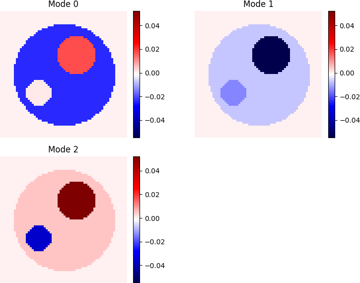
DMD Modes of Simulated Cell — **Figure:** The first three DMD modes extracted from the FLIP simulation.

Mode Interpretation

Mode 0: captures the global bleaching behavior. The cytoplasm appears dark blue, indicating strong decay. The aggregate shows values close to zero — meaning it remains relatively constant — while the nucleus is light red, indicating a slightly slower decay or even minor replenishment. This mode reflects the dominant dynamic, and if you look further ahead this is just like we would expect with the linear system that it is based on. Cytoplasm is losing, aggregates stays the same and nucleus is gaining.

Mode 1:Here we see that all three compartments are losing wight. This is a slower dynamic, and when mode 0, the most dominant mode, has been going then there are unequal weights in each of the compartments, so even though that the dynamics of the linear system tells that some compartments are gaining then at some time they have too much and are now losing. Here we can see that the nucleus are losing much and the aggregates as well.

Mode 2: Here we see what happens at the latest times. The background indicates zero, thus we can see that the cytoplasm is gaining weight (It is slightly darker red than the background), and the nucleus is gaining weight the aggregat loses weight here. We also notice that each mode correspond to a different compartment losing weight.

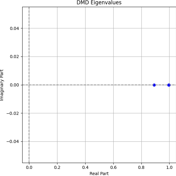
DMD Eigenvalues from FLIP Simulation — **Figure:** DMD eigenvalues plotted in the complex plane and converted to continuous time. Each eigenvalue describes how quickly a mode decays.

The eigenvalues confirm our interpretation. We convert the discrete-time DMD eigenvalues to continuous time using: \[ \omega = \frac{\log(\lambda)}{\Delta t}, \quad \Delta t = 0.5 \]

  Eigenvalues (ω): [-0.230, -0.011, -0.005]

The largest (most negative) value corresponds to rapid bleaching in the cytoplasm (Mode 0), while the slower eigenvalues correspond to the dynamics of the nucleus and aggregate (Modes 1 and 2). All values are real and negative — indicating monotonic decay with no oscillations.

In summary, this example shows that DMD is capable of uncovering hidden compartments and dynamic behavior from image sequences alone — making it a promising technique for analyzing fluorescence recovery and transport in cells.

Validating DMD with Analytical Eigenvalues

One of the most important questions when applying DMD to biological or physical systems is whether it captures the true underlying dynamics. In this section, we validate our data-driven results by comparing DMD eigenvalues to the exact eigenvalues obtained from the known governing equations of our FLIP simulation.

Since the model we simulated is fully known and linear, we can analytically derive the Jacobian matrix \( A \) describing the evolution of fluorescence intensities \( F_c, F_n, F_a \) in the cytoplasm, nucleus, and aggregate: \[ \frac{d\mathbf{F}}{dt} = A \mathbf{F} \] where the form of \( A \) depends on whether the aggregate is included in the simulation.

Theoretical Model (With Aggregate)

When the aggregate is included, the system is described by three coupled ODEs with the following structure:

\[ \begin{aligned} \frac{dF_c}{dt} &= k_1 F_n - k_2 F_c - \beta F_c - k_3 F_c + k_4 F_a \\ \frac{dF_n}{dt} &= -k_1 F_n + k_2 F_c \\ \frac{dF_a}{dt} &= k_3 F_c - k_4 F_a \end{aligned} \]

With the parameters used in our simulation:

  k₁ = 0.025 k₂ = 0.15 β = 0.05 k₃ = 0.01 k₄ = 0.01

The Jacobian matrix becomes:

\[ A = \begin{bmatrix} -0.21 & 0.025 & 0.01 \\ 0.15 & -0.025 & 0 \\ 0.01 & 0 & -0.01 \end{bmatrix} \]

Computing the eigenvalues of this matrix gives us the true continuous-time dynamics:

  Analytical eigenvalues: −0.229, −0.011, −0.005

Comparison with DMD Eigenvalues

DMD estimates a discrete-time evolution matrix \( \tilde{A} \) from snapshot data. To compare it with our continuous model, we convert the eigenvalues using:

\[ \omega_i = \frac{\log(\lambda_i)}{\Delta t} \quad \text{with} \quad \Delta t = 0.5 \]

In our FLIP DMD experiment, the extracted eigenvalues were:

  DMD eigenvalues (ω): −0.230, −0.011, −0.005

These values match almost exactly with the analytical eigenvalues derived from the ODE model. The close correspondence confirms that:

The fast-decaying mode: corresponds to photobleaching in the cytoplasm.
The mid-speed mode: reflects what happens after we change the weight a bit, and release of the nucleus.
The slowest mode: reveals retention and release from the aggregate.

This match is especially impressive given that DMD was applied directly to image data — without prior knowledge of the compartment structure or ODEs.

In conclusion, this experiment shows that DMD not only decomposes spatial dynamics into interpretable modes — it also recovers the correct temporal scales of biological processes. The eigenvalue comparison demonstrates that DMD can uncover the same structure as the governing equations themselves, validating it as a tool for inverse modeling and quantitative cell analysis.

Applying DMD to Experimental FLIP Data

In this final analysis, we turn to real experimental data: a FLIP microscopy video capturing live-cell fluorescence decay over time. The dataset reflects biological transport processes such as diffusion, binding, and compartmental exchange within a single cell after photobleaching.

We process the video into a matrix \( X \in \mathbb{R}^{n \times T} \), where each column corresponds to a vectorized fluorescence frame. Using DMD(svd_rank=0), we apply full-rank Dynamic Mode Decomposition to this spatiotemporal signal.

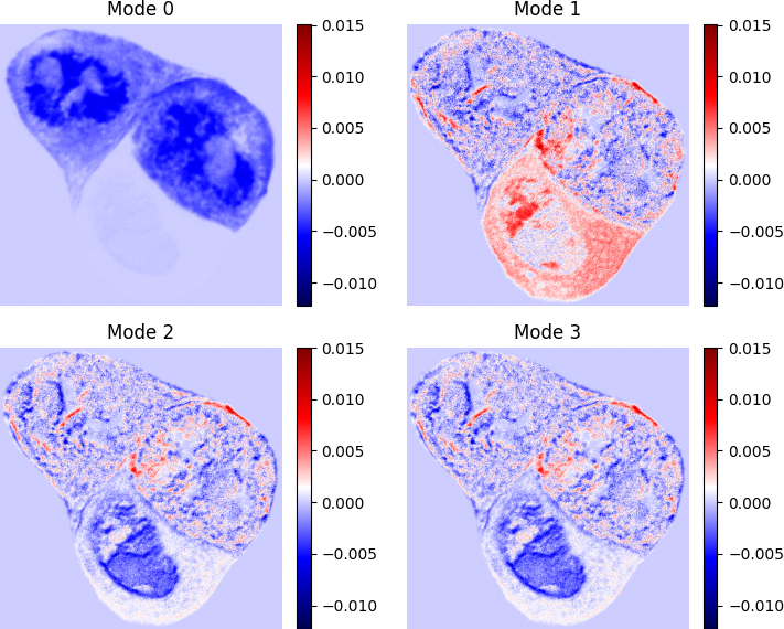
DMD Modes of Real FLIP Data — **Figure:** The first four DMD modes extracted from the experimental FLIP sequence. Red indicates increasing intensity; blue indicates decay.

Interpreting the DMD Modes

Each DMD mode captures a spatial structure associated with a distinct temporal behavior. By examining the patterns of signal change across the cell, we gain insight into the dominant physiological processes:

Mode 0: The first mode is usually the background. This is the mode that does not change during images. As we can see it seem like we have three cells in this image, and the upper and the rightmost cell is the background. This makes sense since we did not bleach here. This also shows that there are not a “fast” connection between the cells, otherwise they would lose their mass when bleaching.
Mode 1:In the leftmost cell, we kind of see three compartments. A nucleus, that I would seperate in the upper and the lower part, and the cytoplasm around the nucleus. We see that the cytoplasm is gaining proteins very uniformly. Then we have the upper section of the nucleus, that gains a lot and more than the cytoplasm. We do not look at the other two cells.
Mode 2: Mode 2 and 3 have the same eigenvalues they just differ in the complex number which are complex conjugate, this can happen using the DMD. Here we have that the lower section of the nucleus is losing quite a bit, and these modes show that while most of the cell is losing the main parts are the lower section and the upper section where the great gain of the protein does not lie.
Mode 3: Shows the same as mode 2.

These modes allow us to spatially resolve how different subcellular compartments behave over time — something that traditional region-averaged analysis often obscures.

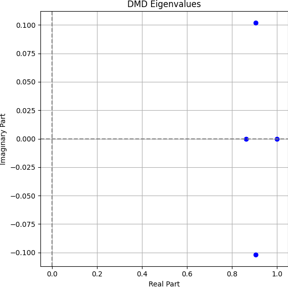
Eigenvalues from Real FLIP DMD — **Figure:** DMD eigenvalues of the experimental FLIP dataset. All values are real and negative, indicating exponential decay of fluorescence.

Interpreting the Eigenvalues

The eigenvalues \( \lambda_i \) extracted from DMD describe the temporal behavior of each mode. For this real cell:

\[ \lambda_1 \approx -0.0027, \quad \lambda_2 \approx -0.298, \quad \lambda_3 \approx -0.186, \quad \lambda_4 \approx -0.186 \]

All eigenvalues are real and negative, consistent with irreversible fluorescence decay. The slower eigenvalue (−0.0027) likely corresponds to mode 1 and the background, since there are not a low of change then we would expect the decay to go very slowly. The faster ones (−0.186 to −0.298) likely reflect photobleaching in the illuminated region and rapid exchange. These show mode 1, the fastest one, where some of the regions are gaining proteins, and then mode 2 and 3 for a slower pace that is losing in the entire cell.

Conclusion: DMD for Quantitative FLIP Analysis

Throughout this project, we demonstrated how Dynamic Mode Decomposition can decompose both simulated and real FLIP microscopy data into coherent spatial structures and interpretable time constants. From blinking Gaussian blobs to biologically realistic transport systems, DMD consistently uncovered dominant dynamics that matched known behavior — including exchange rates, bleaching timescales, and compartmental isolation.

We used a classical implementation of DMD with no modifications: basic SVD truncation, no filtering, and standard numerical precision. However, there is significant room to enhance model fidelity. One could:

Use Tikhonov-regularized DMD for robustness to noise
Include time-delay embeddings to capture nonlinear dynamics
Preprocess data with motion correction or segmentation
Fit the continuous-time model directly via Total Least Squares

In summary, DMD is a powerful, lightweight tool for revealing structure in high-dimensional fluorescence data. Even with minimal assumptions, it provides clear physical interpretations that can guide further modeling and experimentation in live-cell biology.

References

Schmid, P. J. (2010). Dynamic mode decomposition of numerical and experimental data. Journal of Fluid Mechanics, 656, 5–28.
Kutz, J. N., et al. (2016). Dynamic Mode Decomposition: Data-Driven Modeling of Complex Systems. SIAM.
Brunton, S. L., & Kutz, J. N. (2022). Data-Driven Science & Engineering. Cambridge University Press.
pyDMD GitHub: https://github.com/mathLab/PyDMD
Wüstner, D. (2022). Dynamic Mode Decomposition of Fluorescence Loss in Photobleaching Microscopy Data for Model‑Free Analysis of Protein Transport and Aggregation in Living Cells. Sensors, 22(13), Article 4731. https://doi.org/10.3390/s22134731