
SINDy – Sparse Identification of Nonlinear Dynamics
Many natural phenomena are governed by deterministic rules — often expressed as differential equations. Yet in complex or chaotic systems, we rarely know these equations in closed form. The goal of this project is to investigate whether it's possible to automatically discover these governing equations directly from observed data, using sparse regression techniques. Our focus is the SINDy method (Sparse Identification of Nonlinear Dynamical Systems), which aims to balance accuracy and interpretability by identifying only a small number of active terms in a candidate function library.
We explore this approach using four well-known chaotic systems: Rössler, Shimizu–Morioka, Thomas, and Chen. Each provides a different challenge in terms of dimensionality, dynamics, and nonlinearity. We simulate these systems numerically, generate synthetic data, and apply SINDy to infer the underlying equations — both in noise-free and noisy settings.
Beyond evaluating accuracy, we ask: How does chaos affect identifiability? And: What role does sampling, noise, and model selection play in uncovering the dynamics? These questions are central to the practical use of machine learning in scientific discovery.
Theoretical Background: Sparse Identification of Dynamics
The Sparse Identification of Nonlinear Dynamical Systems (SINDy) algorithm is a data-driven method for discovering governing equations of dynamical systems based purely on observations of the system’s evolution. The central idea behind SINDy is that many physical systems, although possibly complex in behavior, are often governed by a small number of underlying mechanisms. Mathematically, this means that the true dynamics can be expressed as a sparse combination of functions from a larger library.
Consider a dynamical system with state vector \( \mathbf{x}(t) \in \mathbb{R}^n \) evolving in time according to an unknown differential equation:
where \( \mathbf{f} \) is a (possibly nonlinear) function that we wish to identify. Given a time series \( \mathbf{x}(t_0), \mathbf{x}(t_1), \ldots, \mathbf{x}(t_m) \), we numerically approximate the time derivatives \( \dot{\mathbf{x}} \) and seek a representation of each component \( \dot{x}_i \) as a linear combination of basis functions.
To this end, we construct a feature matrix \( \Theta(\mathbf{x}) \in \mathbb{R}^{m \times p} \) whose columns are nonlinear candidate functions evaluated at the observed data points. Typical entries in \( \Theta(\mathbf{x}) \) may include constant terms, polynomials, trigonometric functions, or other nonlinearities, such as:
The key assumption is that each derivative \( \dot{x}_i \) depends only on a few of these functions. Thus, we seek a sparse coefficient vector \( \boldsymbol{\xi}_i \in \mathbb{R}^p \) such that:
where \( \varepsilon \) is a residual error term. Stacking the equations for all \( n \) variables, we obtain the full system in matrix form:
where \( \dot{\mathbf{X}} \in \mathbb{R}^{m \times n} \) contains the time derivatives and \( \Xi \in \mathbb{R}^{p \times n} \) is the sparse coefficient matrix. The task is now to determine \( \Xi \) such that most of its entries are exactly zero, retaining only the significant terms.
This is achieved through sparse regression techniques. A simple and effective approach is the Sequentially Thresholded Least Squares (STLSQ) algorithm, which alternates between fitting a least-squares solution and zeroing out small coefficients below a given threshold. This iterative process converges to a compact model that balances accuracy with parsimony, uncovering interpretable equations that reflect the intrinsic structure of the underlying system.
Hello World! — The Lorenz System
To demonstrate how SINDy works in practice, we begin with a classic benchmark from the study of chaos: the Lorenz system. Originally derived as a simplified model for atmospheric convection, the Lorenz equations are now a textbook example of deterministic chaos in continuous dynamical systems.
The Lorenz system consists of three coupled nonlinear differential equations:
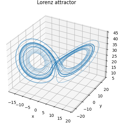
Using standard parameters \( \sigma = 10 \), \( \rho = 28 \), and \( \beta = \frac{8}{3} \), the system exhibits chaotic dynamics: sensitive dependence on initial conditions, bounded trajectories, and a fractal-like attractor in phase space. This attractor forms a twisted double-lobed structure where solutions appear to jump unpredictably between lobes — despite being fully deterministic.
We numerically integrate the Lorenz system using SciPy's solve_ivp, starting from an
initial condition \( (-8, 7, 27) \) and sampling over 25 seconds with 10,000 time points.
The resulting trajectory is shown below:
With this dataset in hand, we now apply SINDy to learn the underlying equations directly from the simulated data.
Thanks to the PySINDy library, the process is remarkably straightforward:
        import pysindy as ps

        model = ps.SINDy()
        model.fit(X, sol.t)
        model.print()
The learned equations are:
        (x0)' = -10.003 x0 + 10.003 x1
        (x1)' = 27.804 x0 + -0.953 x1 + -0.994 x0 x2
        (x2)' = -2.667 x2 + 0.999 x0 x1
These results closely match the original Lorenz parameters. Despite being learned purely from data, the identified model captures both the structure and coefficients of the true system to high precision.
To assess the model’s predictive performance, we simulate both the original system and the learned SINDy model from the same initial condition. The trajectories for \( x(t) \) are plotted below:
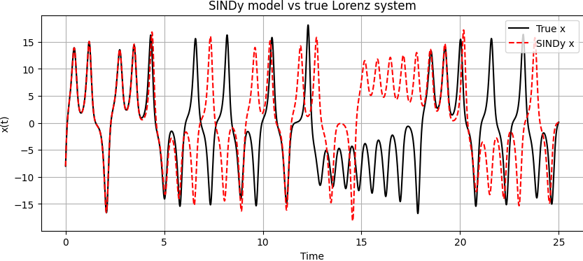
The short-term agreement confirms that the SINDy model captures the system’s essential dynamics. The long-term divergence is expected: in chaotic systems, small differences in parameters or initial conditions grow exponentially over time. What matters is that the learned model correctly reproduces the qualitative structure — the attractor geometry, the feedback terms, and the governing interactions.
Under the Hood: Building SINDy Ourselves
To understand how SINDy works internally, let us step through the main components of the algorithm using the Lorenz system.
This helps demystify the magic behind model.fit(X, t) and shows how the method discovers equations from data.
We start with our data — a matrix \( X \in \mathbb{R}^{m \times n} \) containing \( m \) time samples of the system’s state \( \mathbf{x}(t) \in \mathbb{R}^n \). But SINDy doesn’t learn from position alone — it needs the rate of change, the time derivatives \( \dot{\mathbf{x}}(t) \).
Since we don’t have analytical derivatives, we compute them numerically. The simplest method is finite differences: for small time steps \( \Delta t \),
This gives us \( \dot{X} \), a matrix of the same shape as \( X \).
Libraries like pysindy provide smoother estimators, but the principle is the same.
The next step is to build a function library \( \Theta(X) \). This is a transformation of our data into many nonlinear combinations — the candidate right-hand-side terms in the differential equations. We’ll use all polynomial combinations up to degree 3.
As a small example: suppose \( x = 2 \) and \( y = -1 \). Then the second-degree polynomial library might include:
The full library \( \Theta(X) \in \mathbb{R}^{m \times p} \) evaluates such terms for all time points. In practice, this step is handled by PySINDy, but we can inspect its shape and content directly.
Now comes the key part: solving the sparse regression problem \( \dot{X} = \Theta(X) \cdot \Xi \). The matrix \( \Xi \) contains the coefficients of each function in the library. Most entries should be zero — only a few terms are active in each equation.
We use the STLSQ algorithm (Sequentially Thresholded Least Squares), which starts by fitting a standard least-squares solution, then iteratively sets small coefficients to zero and refits only the remaining ones. Here is a simplified version:
        def STLSQ(Theta, dXdt, threshold=0.1, max_iter=10):
            Xi = np.linalg.lstsq(Theta, dXdt, rcond=None)[0]
            for _ in range(max_iter):
                small_inds = np.abs(Xi) < threshold
                Xi[small_inds] = 0
                for i in range(dXdt.shape[1]):
                    big_inds = ~small_inds[:, i]
                    if np.any(big_inds):
                        Xi[big_inds, i] = np.linalg.lstsq(Theta[:, big_inds], dXdt[:, i], rcond=None)[0]
            return Xi
The threshold parameter controls sparsity — if set too high, important terms may be removed.
If too low, the model becomes dense and overfits. With threshold = 0.1,
the recovered coefficient matrix looks like:
        [[  0.           0.           0.        ]
        [-10.003        27.804        0.        ]
        [ 10.003        -0.953        0.        ]
        [  0.            0.          -2.667      ]
        [  0.            0.           0.999      ]
        [  0.           -0.994        0.        ]]
This matrix corresponds to the learned equations:
These match the original Lorenz system, and we obtained them using our own code. For convenience, we still use PySINDy’s feature library and differentiation tools, but the core regression is fully transparent.
Subsampling Across Chaotic Systems: How Much Data is Enough?
A key question in data-driven modeling of chaotic systems is: how much data is needed to recover the correct dynamics? To answer this, we compare how well the Sparse Identification of Nonlinear Dynamical Systems (SINDy) framework performs on four different chaotic systems under varying amounts of available data. These systems differ in complexity and chaotic behavior, measured by their largest Lyapunov exponent.
We generate clean simulation data for each system and then subsample the time series to simulate lower data availability.
Subsampling here refers to reducing the number of timepoints used for fitting, for instance by taking every k-th point
or slicing the first N values from the total trajectory. We define a successful identification as finding exactly the correct terms in the governing equations — no more, no less.
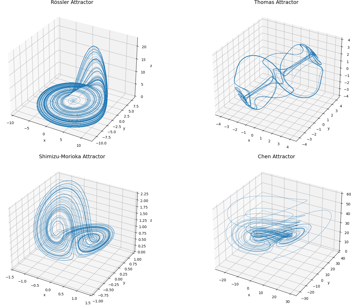
The Four Chaotic Systems
Rössler System
This system generates a smooth spiral-like attractor. It is considered weakly chaotic, with a Lyapunov exponent of approximately 0.07. Because of its simple geometry and low-dimensional structure, it serves as a benchmark for easy identification.
Thomas Cyclic System
This system involves cyclic exchange of energy between dimensions through sine terms. It has a Lyapunov exponent near 0.16 and features toroidal trajectories. Crucially, the use of sine makes it invisible to purely polynomial libraries.
Shimizu–Morioka System
The Shimizu system has moderate chaos with a Lyapunov exponent of approximately 0.10. Its dynamics are dominated by polynomial interactions, which makes it an ideal candidate for a polynomial basis.
Chen System
The Chen system is strongly chaotic, with a Lyapunov exponent near 2.0. Despite being polynomial, its sensitivity to initial conditions and fast divergence make it difficult to identify even under favorable conditions.
Identification Results
For each system, we tested identification using two types of libraries:
a polynomial basis up to degree 5, and an extended basis including trigonometric functions.
The systems were fitted using pysindy.SINDy with finite-difference differentiation, and
a sparsity threshold of 0.1.
         RÖSSLER (λ₁ ≈ 0.07)
        PolyLib:    @10k (1.52%),  @5k (6.38%),  ≤1k
        TrigLib:    @10k,  @5k,  ≤1k

         THOMAS (λ₁ ≈ 0.16)
        PolyLib:    all datapoints
        TrigLib:    @10k–500,  ≤200

         SHIMIZU–MORIOKA (λ₁ ≈ 0.10)
        PolyLib:    @10k–5k,  ≤1k
        TrigLib:    all datapoints

         CHEN (λ₁ ≈ 2.0)
        PolyLib:    all datapoints
        TrigLib:    all datapoints
These results reveal a clear pattern: systems with lower Lyapunov exponents (less chaos) require fewer data points for successful identification. Rössler and Shimizu, for example, were accurately recovered with just 5,000 points. In contrast, the Chen system could not be correctly identified even with 10,000 samples, due to its extreme sensitivity and dynamic richness.
Interestingly, the Thomas system was only identifiable when a trigonometric library was used. This highlights an important consideration: correct model structure must be expressible in the chosen function library. Even abundant data will not help if key features (like sine terms) are missing from the representation.
In conclusion, successful sparse identification depends on both the chaotic intensity of the system and the expressiveness of the feature library. With sufficiently smooth dynamics and appropriate bases, sparse recovery is remarkably effective — even from as few as 1,000 time samples.
Robustness to Noise: Can We Still Discover the Dynamics?
Real-world measurements are rarely noise-free. Even the most precise experimental data contain fluctuations due to sensor error, digitization, or environmental interference. To test the robustness of sparse identification, we revisit our four chaotic systems and now add Gaussian noise to the simulated trajectories.
Noise is added to the state vector \( \mathbf{x}(t) \) such that:
\[
\mathbf{x}_{\text{noisy}}(t) = \mathbf{x}(t) + \mathcal{N}(0, \sigma^2)
\]
where \( \sigma \) is a percentage of the standard deviation of the signal (here set to 1% of the signal amplitude). We then perform identification exactly as before using pysindy with polynomial libraries.
Due to the destabilizing nature of noise — especially in numerical differentiation — even small levels of perturbation drastically degrade performance. This test therefore acts as a stress test for both the numerical methods and the sparsity assumption in SINDy.
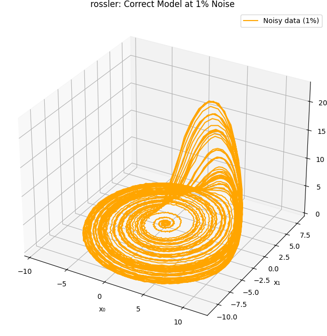
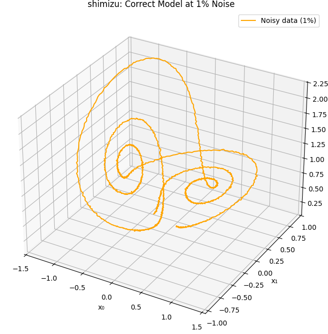
Among all tested systems, only the Rössler and Shimizu–Morioka systems allowed correct structural recovery at 1% noise. This is consistent with their lower Lyapunov exponents and smoother attractors, which provide better tolerance to perturbations.
In contrast, the Thomas and Chen systems completely failed under noise. The Thomas system’s sensitivity to sine distortion, and the Chen system’s inherently unstable dynamics, make them especially vulnerable. This suggests that robustness to noise correlates strongly with both model simplicity and chaotic strength.
These findings emphasize the importance of denoising strategies and robust differentiation methods in real applications. While SINDy is powerful, its accuracy is tightly coupled to the quality of the input data.
Conclusion
In this project, we explored the Sparse Identification of Nonlinear Dynamical Systems (SINDy) method as a tool for learning governing equations directly from data. Through simulation and systematic testing on a range of chaotic systems — Rössler, Thomas, Shimizu–Morioka, and Chen — we demonstrated both the potential and limitations of the technique.
Our results show that SINDy is indeed capable of uncovering accurate models when the data is clean, well-sampled, and when the correct function library is used. However, the method is also highly sensitive to noise, sampling rate, and model mismatch. For instance, when sinusoidal terms were absent from the library, the Thomas system could not be recovered, and under even 1% noise, only the Rössler and Shimizu–Morioka systems remained identifiable.
Despite these challenges, we did not attempt extensive parameter tuning. The thresholding parameter in the STLSQ algorithm, the choice of optimizer, the structure of the function library, and the differentiation method were all left at their defaults. Each of these elements could be optimized further — either through manual tuning, cross-validation, or automatic model selection strategies — to significantly improve robustness.
In practice, applying SINDy effectively requires both domain knowledge and algorithmic experimentation. But when tuned correctly, SINDy offers a compelling bridge between data-driven modeling and interpretable, physically grounded differential equations — even for complex nonlinear systems.
References
- Brunton, S. L., Proctor, J. L., & Kutz, J. N. (2016). Discovering governing equations from data by sparse identification of nonlinear dynamical systems. PNAS, 113(15), 3932–3937. DOI
- Kaheman, K., Kutz, J. N., & Brunton, S. L. (2022). SINDy sampling strategies. arXiv:2202.11638. Link
- De Silva, B. M., Champion, K., & Brunton, S. L. (2020). Multiscale modeling of dynamical systems using sparse identification. Phys. Rev. E, 101(1), 013311. DOI
- Kaptanoglu, A. A., et al. (2022). PySINDy: A Python package for sparse identification of nonlinear dynamical systems. JOSS, 7(76), 4596. DOI
- PySINDy GitHub: https://github.com/dynamicslab/pysindy